Freezing Params Across Fits

A common two-stage workflow: fit a wide wavelength range to constrain the continuum and kinematics, then re-fit a subset of lines with those parameters frozen to their posterior values.

In this tutorial we simulate a spectrum containing H\(\alpha\) + [NII]\(\lambda\lambda\)6549, 6585 + [SII]\(\lambda\lambda\)6717, 6731 on a sloping linear continuum.

• Fit 1 — full line set (Ha + NII + SII), all parameters free. fit() automatically attaches log_prob (log joint) and log_likelihood to the returned sample dict.

• Fit 2 — Ha + NII only (SII dropped). Continuum and kinematics are frozen from Fit 1 via freeze_from_samples(), which now returns all parameters — including those that were already Fixed (such as norm_wav_a) — so no manual lookup of region centres is needed.

Key design choices demonstrated:

• Reuse the same Spectra object for both fits. compute_scales is called once with the first (most complete) configuration. Recomputing with a different line set would produce a different continuum_scale, making the frozen amplitude parameters physically inconsistent between fits.

• The naive from_lines centre for Ha + NII alone (~6568 A) differs by ~79 A from Fit 1’s centre (~6647 A). Using frozen['norm_wav_a'] directly pins the correct reference wavelength without any manual arithmetic.

Step 0 — Imports and Setup

import astropy.units as u
import numpy as np
from matplotlib import pyplot

from unite import continuum, line, model, prior, results, spectrum
from unite.instrument.generic import SimpleDisperser
from unite.results import count_parameters

pyplot.style.use('unite.mplstyle')

Step 1 — Simulate a Spectrum

A 600-pixel synthetic spectrum (6200-6800 A) with narrow Ha + [NII] + [SII] on a steeply sloping linear continuum. The slope is steep enough that an 80 A shift in normalization wavelength moves the continuum level by ~3 counts (about 1 sigma), making the norm_wav trap visible in the residuals.

rng = np.random.default_rng(42)

WL_MIN, WL_MAX, N_PIX = 6200.0, 6800.0, 600
wl = np.linspace(WL_MIN, WL_MAX, N_PIX)
dlam_pix = (WL_MAX - WL_MIN) / (N_PIX - 1)

disperser = SimpleDisperser(wavelength=wl * u.AA, R=1200.0, name='grism')

c_kms = 299792.458
lsf_fwhm_ha = 6563.0 / 1200.0
fwhm_narrow_aa = np.sqrt((6563.0 * 200.0 / c_kms) ** 2 + lsf_fwhm_ha**2)
sigma_narrow = fwhm_narrow_aa / (2 * np.sqrt(2 * np.log(2)))

true_cont_level = 20.0
true_slope = 0.04  # counts / Angstrom  (1e-17 erg/s/cm2/AA units)
true_continuum = true_cont_level + true_slope * (wl - 6550.0)


def g(center: float) -> np.ndarray:
    return np.exp(-0.5 * ((wl - center) / sigma_narrow) ** 2)


true_lines = (
    60.0 * g(6563.0)  # Ha
    + 15.0 * g(6549.0)  # NII 6549
    + 45.0 * g(6585.0)  # NII 6585
    + 10.0 * g(6717.0)  # SII 6717
    + 15.0 * g(6731.0)  # SII 6731
)
noise_sigma = 3.0

flux_arr = (true_lines + true_continuum + rng.normal(0, noise_sigma, N_PIX)) * 1e-17
error_arr = np.full(N_PIX, noise_sigma * 1e-17)
flux_q = flux_arr * u.erg / u.s / u.cm**2 / u.AA
error_q = error_arr * u.erg / u.s / u.cm**2 / u.AA

half = 0.5 * dlam_pix
spec = spectrum.from_edges(
    (wl - half) * u.AA, (wl + half) * u.AA, flux_q, error_q, disperser, name='grism'
)

fig, ax = pyplot.subplots(figsize=(10, 4))
ax.step(wl, flux_arr * 1e17, where='mid', color='k', lw=0.7)
ax.set(
    xlabel=r'$\lambda$ [\AA]',
    ylabel=r'$f_\lambda$ [$10^{-17}$ erg s$^{-1}$ cm$^{-2}$ \AA$^{-1}$]',
    title=r'Synthetic Ha + [NII] + [SII] on a sloping continuum',
)
pyplot.tight_layout()
# pyplot.show()

Step 2 — Fit 1: Full Line Set, All Parameters Free

Note on the Spectra object. We create spectra once and call compute_scales once. Fit 2 will re-use the same object — calling prepare again with a different line config is fine, but calling compute_scales again would produce a different continuum_scale (because line masking differs without SII), making the frozen scale_a value physically inconsistent.

NumPyro site names — for reference:

• Redshift('narrow') → z_narrow

• FWHM('narrow') → fwhm_gauss_narrow

• Flux('Ha') → flux_Ha; Flux('NII') → flux_NII

• Flux('SII') → flux_SII

• Auto-generated continuum tokens → scale_a, angle_a, norm_wav_a

z_narrow = line.Redshift('narrow', prior=prior.Uniform(-0.001, 0.001))
fwhm_narrow = line.FWHM('narrow', prior=prior.Uniform(50, 500))

lc = line.LineConfiguration()
lc.add_line(
    'Ha',
    6563.0 * u.AA,
    profile='Gaussian',
    redshift=z_narrow,
    fwhm_gauss=fwhm_narrow,
    flux=line.Flux(prior=prior.Uniform(0, 3)),
)
lc.add_lines(
    'NII',
    np.array([6549.0, 6585.0]) * u.AA,
    profile='Gaussian',
    redshift=z_narrow,
    fwhm_gauss=fwhm_narrow,
    strength=[1.0, 3.0],
    flux=line.Flux(prior=prior.Uniform(0, 3)),
)
lc.add_lines(
    'SII',
    np.array([6717.0, 6731.0]) * u.AA,
    profile='Gaussian',
    redshift=z_narrow,
    fwhm_gauss=fwhm_narrow,
    strength=[1.0, 1.5],
    flux=line.Flux(prior=prior.Uniform(0, 3)),
)

cc = continuum.ContinuumConfiguration.from_lines(
    lc.centers, width=15_000 * u.km / u.s, form=continuum.Linear()
)

spectra = spectrum.Spectra([spec], redshift=0.0)
filtered_lc, filtered_cc = spectra.prepare(lc, cc)
spectra.compute_scales(
    filtered_lc,
    filtered_cc,
    line_mask_width=3_000 * u.km / u.s,
    box_width=2_000 * u.km / u.s,
)

print(
    f'Fit 1 continuum region: [{filtered_cc[0].low:.1f}, {filtered_cc[0].high:.1f}] AA'
)
print(f'Fit 1 norm_wav (region center): {filtered_cc[0].center:.1f} AA')
print(
    f'Continuum scale: {spectra.continuum_scale:.4g}  (will not be recomputed for Fit 2)'
)

# ModelBuilder.fit() automatically attaches log_prob and log_likelihood.
samples1, args1 = model.ModelBuilder(filtered_lc, filtered_cc, spectra).fit(
    num_warmup=500, num_samples=1000, num_chains=2, progress_bar=False
)

pct = np.array([0.16, 0.5, 0.84])
t1 = results.make_parameter_table(samples1, args1, percentiles=pct)
print('\nFit 1 results (includes log_prob and log_likelihood columns):')
print(t1)

Fit 1 continuum region: [6385.2, 6899.4] AA
Fit 1 norm_wav (region center): 6642.3 AA
Continuum scale: 1.896e-16 erg / (Angstrom s cm2)  (will not be recomputed for Fit 2)
/home/docs/checkouts/readthedocs.org/user_builds/unite/checkouts/v3.3.0/unite/model.py:852: UserWarning: There are not enough devices to run parallel chains: expected 2 but got 1. Chains will be drawn sequentially. If you are running MCMC in CPU, consider using `numpyro.set_host_device_count(2)` at the beginning of your program. You can double-check how many devices are available in your system using `jax.local_device_count()`.
  mcmc = infer.MCMC(

Fit 1 results (includes log_prob and log_likelihood columns):
percentile        z_narrow        ...      log_prob        log_likelihood
                                  ...
---------- ---------------------- ... ------------------ ------------------
      0.16 -1.109138326602633e-05 ... 230.49674992486462  248.1217370146355
       0.5 1.4098528330208637e-07 ... 232.44481619376845 250.05267567836447
      0.84 1.1441627699851184e-05 ... 233.91232161883661 251.54135294668404

Step 3 — Freeze Parameters with freeze_from_samples

freeze_from_samples() now returns every parameter in the model — including those that were already Fixed. norm_wav_a (which Linear auto-fixes to the region centre) therefore appears in frozen with its exact value, so Fit 2 can pin it without any manual lookup.

The default cenfunc='median' summarises each free parameter’s posterior independently. For correlated parameters (e.g. continuum scale_a and angle_a), the joint MAP sample is more consistent:

frozen = results.freeze_from_samples(samples1, args1)
print('Frozen site names:', sorted(frozen.keys()))
print(f'norm_wav_a = {frozen['norm_wav_a'].resolved_value({}):.1f} AA')

# MAP alternative: use the sample with the highest log posterior.
# cenfunc='map' requires 'log_prob' in samples, which ModelBuilder.fit() always provides.
frozen_map = results.freeze_from_samples(samples1, args1, cenfunc='map')
print(
    f'MAP scale_a = {frozen_map['scale_a'].resolved_value({}):.4f}  '
    f'(median = {frozen['scale_a'].resolved_value({}):.4f})'
)

Frozen site names: ['angle_a', 'flux_Ha', 'flux_NII_6549', 'flux_SII_6717', 'fwhm_gauss_narrow', 'norm_wav_a', 'scale_a', 'z_narrow']
norm_wav_a = 6642.3 AA
MAP scale_a = 1.2382  (median = 1.2423)

Step 4 — Build Fit 2: Ha + NII Only, Continuum Frozen

The norm_wav trap. Because Fit 2 drops [SII], a naive from_lines call on just Ha + NII would produce a narrower merged region (~6385-6750 A) centred at ~6568 A — about 79 A away from Fit 1’s norm_wav of ~6647 A. Freezing scale_a at a wrong norm_wav introduces a flat continuum offset of tan(angle_a) * continuum_scale * delta_norm_wav.

With freeze_from_samples now returning norm_wav_a, the fix is simply to pass frozen['norm_wav_a'] to the new region — no arithmetic required.

lc2 = line.LineConfiguration()
z_narrow2 = line.Redshift('narrow', prior=frozen['z_narrow'])
fwhm_narrow2 = line.FWHM('narrow', prior=frozen['fwhm_gauss_narrow'])
lc2.add_line(
    'Ha',
    6563.0 * u.AA,
    profile='Gaussian',
    redshift=z_narrow2,
    fwhm_gauss=fwhm_narrow2,
    flux=line.Flux(prior=prior.Uniform(0, 3)),
)
lc2.add_lines(
    'NII',
    np.array([6549.0, 6585.0]) * u.AA,
    profile='Gaussian',
    redshift=z_narrow2,
    fwhm_gauss=fwhm_narrow2,
    strength=[1.0, 3.0],
    flux=line.Flux(prior=prior.Uniform(0, 3)),
)

# What from_lines alone would give — demonstrating the wrong centre.
cc2_naive = continuum.ContinuumConfiguration.from_lines(
    lc2.centers, width=15_000 * u.km / u.s, form=continuum.Linear()
)
naive_norm_wav = cc2_naive[0].center
fit1_norm_wav = frozen['norm_wav_a'].resolved_value({})
delta_nw = naive_norm_wav - fit1_norm_wav
median_angle = float(np.median(samples1['angle_a']))
expected_offset = np.tan(median_angle) * float(spectra.continuum_scale.value) * delta_nw

print(f'Fit 1  norm_wav: {fit1_norm_wav:.1f} AA  (from frozen dict)')
print(f'Naive Fit 2 norm_wav: {naive_norm_wav:.1f} AA  (delta = {delta_nw:+.1f} AA)')
print(
    f'Expected continuum offset from wrong norm_wav: {expected_offset:.2g} '
    f'{spectra.continuum_scale.unit}'
)

# Correct: pin norm_wav to the Fit 1 value via frozen['norm_wav_a'].
frozen_region = continuum.ContinuumRegion(
    cc2_naive[0].low * cc2_naive[0].unit,
    cc2_naive[0].high * cc2_naive[0].unit,
    form=continuum.Linear(),
    params={
        'scale': continuum.Scale(prior=frozen['scale_a']),
        'angle': continuum.ContShape(prior=frozen['angle_a']),
        'norm_wav': continuum.NormWavelength(prior=frozen['norm_wav_a']),
    },
)
cc2 = continuum.ContinuumConfiguration([frozen_region])

Fit 1  norm_wav: 6642.3 AA  (from frozen dict)
Naive Fit 2 norm_wav: 6567.5 AA  (delta = -74.8 AA)
Expected continuum offset from wrong norm_wav: -2.9e-17 erg / (Angstrom s cm2)

Step 5 — Fit 2: Lines Only

Re-prepare on the same spectra object — scales are unchanged. Only Ha and NII fluxes are free.

filtered_lc2, filtered_cc2 = spectra.prepare(lc2, cc2)

print(
    f'Fit 1 free parameters: {count_parameters(model.ModelBuilder(filtered_lc, filtered_cc, spectra).build()[0], args1)}'
)

samples2, args2 = model.ModelBuilder(filtered_lc2, filtered_cc2, spectra).fit(
    num_warmup=300, num_samples=800, num_chains=2, progress_bar=False
)

t2 = results.make_parameter_table(samples2, args2, percentiles=pct)
print('\nFit 2 results (SII dropped, continuum + kinematics frozen):')
print(t2)

Fit 1 free parameters: 7

Fit 2 results (SII dropped, continuum + kinematics frozen):
percentile        z_narrow        ...      log_prob       log_likelihood
                                  ...
---------- ---------------------- ... ----------------- -----------------
      0.16 1.4098528330208637e-07 ... 83.50360033126587 90.78382634503714
       0.5 1.4098528330208637e-07 ... 84.62718408748731 91.91117819204838
      0.84 1.4098528330208637e-07 ... 85.13473769985062   92.416007472979

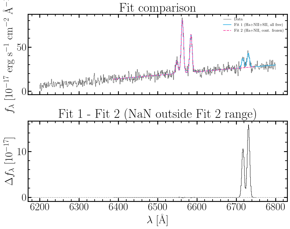
Step 6 — Compare the Two Fits

Ha and NII fluxes should agree between fits. The frozen continuum sits correctly because norm_wav is preserved. [SII] residuals in Fit 2 are expected — those lines are not in the model.

spectra_tables1 = results.make_spectra_tables(
    samples1, args1, insert_nan=True, percentiles=pct
)
spectra_tables2 = results.make_spectra_tables(
    samples2, args2, insert_nan=True, percentiles=pct
)

tab1 = spectra_tables1['grism']
tab2 = spectra_tables2['grism']
wl1 = tab1['wavelength']
wl2 = tab2['wavelength']

fig, axes = pyplot.subplots(2, 1, figsize=(10, 8), sharex=True)

ax = axes[0]
ax.step(wl, flux_arr * 1e17, where='mid', color='k', lw=0.7, alpha=0.7, label='Data')
ax.step(
    wl1,
    tab1['model_total'][:, 1].value * 1e17,
    where='mid',
    color='C0',
    lw=1.5,
    label='Fit 1 (Ha+NII+SII, all free)',
)
ax.step(
    wl2,
    tab2['model_total'][:, 1].value * 1e17,
    where='mid',
    color='C1',
    lw=1.5,
    ls='--',
    label='Fit 2 (Ha+NII, cont. frozen)',
)
ax.set(
    ylabel=r'$f_\lambda$ [$10^{-17}$ erg s$^{-1}$ cm$^{-2}$ \AA$^{-1}$]',
    title='Fit comparison',
)
ax.legend(fontsize=9)

ax = axes[1]
# Fit 2 may cover a different wavelength range; interpolate its model onto
# Fit 1's grid so the difference is defined everywhere, with NaN outside Fit 2.
m2_on_wl1 = np.interp(
    wl1.value, wl2.value, tab2['model_total'][:, 1].value, left=np.nan, right=np.nan
)
diff = (tab1['model_total'][:, 1].value - m2_on_wl1) * 1e17
ax.step(wl1, diff, where='mid', color='k', lw=0.8)
ax.axhline(0, ls='--', color='gray', lw=0.8)
ax.set(
    xlabel=r'$\lambda$ [\AA]',
    ylabel=r'$\Delta f_\lambda$ [$10^{-17}$]',
    title='Fit 1 - Fit 2 (NaN outside Fit 2 range)',
)

pyplot.tight_layout()
# pyplot.show()
print('Done.')

Done.