NIRSpec Fitting

In this tutorial we demonstrate how to use unite to fit multiple NIRSpec spectra simultaneously with a shared multi-component emission line model. We use the built-in NIRSpec support in unite to load spectra directly from the Dawn JWST Archive (DJA).

We fit H\(\alpha\), H\(\beta\), and [OIII] with a narrow + broad decomposition simultaneously across the PRISM and G395M gratings. We are fitting RUBIES-UDS-807469 at \(z \approx 6.78\), a little red dot (LRD) from the RUBIES survey with broad Balmer lines.

Step 0 — Imports and Setup

We import the necessary libraries and set a plotting style for the tutorial.

import astropy.units as u
import jax
import jax.numpy as jnp
from matplotlib import pyplot
from numpyro import infer, optim

from unite import continuum, instrument, line, model, prior, results, spectrum
from unite.instrument import nirspec

pyplot.style.use('unite.mplstyle')

Step 1 — Configure the Dispersers

unite ships with built-in calibrations for all NIRSpec gratings. We attach calibration tokens directly to each disperser object:

• RScale — multiplicative resolution scale (shared across both gratings)

• FluxScale — relative flux normalization for G395M vs PRISM

• PixOffset — sub-pixel wavelength shift for G395M

See Instruments & Spectrum Loading for the full disperser and calibration token reference.

In this example we will use the calibration offsets observed in de Graaff et al. (2025) as a guide for setting the priors on these parameters, but they can be freely adjusted as needed. Setting the resolution source (r_source) to ‘point’ assumes the source is a point source centered in the slit.

# First we define a resolution scaling parameter, essentially inflating
# the resolution element to account for uncertainty in source morphology,
# position within the slit
# In this example we share this parameter across both
# Shared resolution scale: same Python object → single model parameter
resolution_scale = instrument.RScale(
    prior=prior.TruncatedNormal(low=0.6, high=1.4, loc=1.0, scale=0.1)
)

# See Fig 8 in de Graaff+ 2025 for typical observed offsets and scatter between PRISM and G395M.
prism_disperser = nirspec.PRISM(
    r_source='point',
    r_scale=resolution_scale,
    pix_offset=instrument.PixOffset(
        prior=prior.TruncatedNormal(low=-0.2, high=0.6, loc=0.2, scale=0.1)
    ),
)

# See Fig 9 in de Graaff+ 2025 for typical observed flux ratios and scatter between PRISM and G395M.
g395m_disperser = nirspec.G395M(
    r_source='point',
    r_scale=resolution_scale,
    flux_scale=instrument.FluxScale(
        prior=prior.TruncatedNormal(low=0.6, high=1.2, loc=0.9, scale=0.1)
    ),
)

# Combine into a single configuration object for convenience
instrument_config = instrument.InstrumentConfig([g395m_disperser, prism_disperser])
# We could also save and load this object for convienience:
# instrument_config.save('filename.yaml')
# instrument_config = instrument.InstrumentConfig.load('filename.yaml')
print(instrument_config)

InstrumentConfig: 2 disperser(s)

  Name   Disperser                r_scale    flux_scale        pix_offset
  -----  -----------------------  ---------  ----------------  ----------------
  G395M  G395M(r_source='point')  r_scale_a  flux_scale_G395M  — (fixed)
  PRISM  PRISM(r_source='point')  r_scale_a  — (fixed)         pix_offset_PRISM

  R Scale:
    r_scale_a  TruncatedNormal(loc=1.0, scale=0.1, low=0.6, high=1.4)

  Flux Scale:
    flux_scale_G395M  TruncatedNormal(loc=0.9, scale=0.1, low=0.6, high=1.2)

  Pix Offset:
    pix_offset_PRISM  TruncatedNormal(loc=0.2, scale=0.1, low=-0.2, high=0.6)

Step 2 — Load the Spectra from DJA

from_DJA() downloads and parses a NIRSpec spectrum directly from an S3 URL. cache=True stores the file locally with astropy so subsequent runs do not re-download.

See Instruments & Spectrum Loading (NIRSpec section) for more details. and Building the Model for how spectra are collected and prepared.

# Systematic redshift
zspec = 6.7754

# Can load the disperser from the object...
g395m_spectrum = spectrum.from_DJA(
    'https://s3.amazonaws.com/msaexp-nirspec/extractions/'
    'rubies-uds42-v4/rubies-uds42-v4_g395m-f290lp_4233_807469.spec.fits',
    disperser=g395m_disperser,
    cache=True,
)
# Or by name from the configuration object
prism_spectrum = spectrum.from_DJA(
    'https://s3.amazonaws.com/msaexp-nirspec/extractions/'
    'rubies-uds42-v4/rubies-uds42-v4_prism-clear_4233_807469.spec.fits',
    disperser=instrument_config['PRISM'],
    cache=True,
)

spectra = spectrum.Spectra([g395m_spectrum, prism_spectrum], redshift=zspec)

Plot the raw spectra to guide our model design.

fig, axes = pyplot.subplots(1, 2, figsize=(12, 7), sharey=True)
fig.subplots_adjust(wspace=0)
for ax in axes:
    for i, s in enumerate(spectra):
        ax.step(
            s.wavelength,
            s.flux,
            where='mid',
            label=s.disperser.name,
            color=f'C{i}',
            alpha=1.0,
        )
    ax.set_xlabel(rf'$\lambda$ (Obs.) [{prism_spectrum.unit:latex}]')
axes[0].set(
    xlim=[0.45 * (1 + zspec), 0.55 * (1 + zspec)],
    ylabel=rf'$f_\lambda$ [{prism_spectrum.flux_unit:latex_inline}]',
    ylim=[0, 18],
)
axes[1].legend()
axes[1].set(xlim=[0.61 * (1 + zspec), 0.7 * (1 + zspec)])
axes[0].set_title(r'H$\beta$ + [OIII] Region', pad=10)
axes[1].set_title(r'H$\alpha$ Region', pad=10)
pyplot.show()

Step 3 — Configure the Emission Lines

We build a narrow + broad + absorption model:

• Narrow: shared redshift z and FWHM narrow across all lines

• Broad: Gaussian profile with FWHM prior that must exceed narrow + 150 km/s

• [OIII] doublet: fixed 1:3 flux ratio enforced via strength

See Line Configuration for the full line and profile reference and Priors for dependent priors and all supported prior types.

# Create an empty configuration
line_configuration = line.LineConfiguration()

# Shared redshift parameter for all lines
# The prior is relative to the input redshift so the configuration can be reused
z_common = line.Redshift('shared', prior=prior.Uniform(-0.005, 0.005))

# First define the narrow redshift and then the broad FWHM with a prior that depends on the narrow FWHM.
# FWHMs are assumed to be in km/s
fwhm_narrow = line.FWHM('narrow', prior=prior.Uniform(100, 500))
fwhm_broad = line.FWHM('broad', prior=prior.Uniform(fwhm_narrow + 150, 5000))

# Add the Balmer lines using
line_configuration.add_line(
    'Ha', 6564.61 * u.AA, profile='Gaussian', redshift=z_common, fwhm_gauss=fwhm_narrow
)
line_configuration.add_line(
    'Hb', 4862.68 * u.AA, profile='Gaussian', redshift=z_common, fwhm_gauss=fwhm_narrow
)

# Add the [OIII] doublet with fixed 1:3 flux ratio using the ``strength`` argument.
# Note, the add_lines function by default assumes shared parameters across all lines.
# This can be changed by passing a list of parameters to a given argument.
line_configuration.add_lines(
    'OIII',
    [4960.295, 5008.24] * u.AA,
    profile='Gaussian',
    redshift=z_common,
    fwhm_gauss=fwhm_narrow,
    strength=[1.0, 3.0],
)

# Broad components
# Note here how we pass two flux parameters to the ``flux`` argument to allow independent broad fluxes for Ha and Hb.
# We are also going to use a different profile for the broad component to demonstrate the flexibility of the line configuration.
line_configuration.add_lines(
    ['Ha_broad', 'Hb_broad'],
    [6564.61, 4862.68] * u.AA,
    profile='Exponential',
    redshift=z_common,
    fwhm_exp=fwhm_broad,  # Not the different parameter name
    flux=[
        line.Flux(prior=prior.Uniform(0, 3)),
        line.Flux(prior=prior.Uniform(0, 3)),
    ],  # Positive fluxes
)

# Inspect the line configuration
print(line_configuration)

LineConfiguration: 6 lines, 6 flux / 1 z / 2 profile params

  Name          Wavelength        Profile   Redshift  Params             Flux/Tau           zorder  Strength
  ------------  ----------------  --------  --------  -----------------  -----------------  ------  --------
  Ha            6564.61 Angstrom  Gaussian  z_shared  fwhm_gauss_narrow  flux_Ha            0       1.00
  Hb            4862.68 Angstrom  Gaussian  z_shared  fwhm_gauss_narrow  flux_Hb            0       1.00
  OIII_4960.3   4960.30 Angstrom  Gaussian  z_shared  fwhm_gauss_narrow  flux_OIII_4960.3   0       1.00
  OIII_5008.24  5008.24 Angstrom  Gaussian  z_shared  fwhm_gauss_narrow  flux_OIII_5008.24  0       3.00
  Ha_broad      6564.61 Angstrom  Laplace   z_shared  fwhm_exp_broad     flux_Ha_broad      0       1.00
  Hb_broad      4862.68 Angstrom  Laplace   z_shared  fwhm_exp_broad     flux_Hb_broad      0       1.00

  Redshift:
    z_shared  Uniform(low=-0.005, high=0.005)

  Params (fwhm_gauss):
    fwhm_gauss_narrow  Uniform(low=100.0, high=500.0)

  Params (fwhm_exp):
    fwhm_exp_broad  Uniform(low=(narrow + 150.0), high=5000.0)

  Flux:
    flux_Ha            Uniform(low=-3.0, high=3.0)
    flux_Hb            Uniform(low=-3.0, high=3.0)
    flux_OIII_4960.3   Uniform(low=-3.0, high=3.0)
    flux_OIII_5008.24  Uniform(low=-3.0, high=3.0)
    flux_Ha_broad      Uniform(low=0.0, high=3.0)
    flux_Hb_broad      Uniform(low=0.0, high=3.0)

Step 4 — Configure the Continuum

Auto-generate independent linear continua around each line group by padding each line center and merging overlapping windows.

See Continuum Configuration for manual regions, other continuum forms (power law, Chebyshev, blackbody, …), and parameter sharing across regions.

cc = continuum.ContinuumConfiguration.from_lines(
    line_configuration.centers,
    width=15_000 * u.km / u.s,  # width of continuum windows around each line center
    form=continuum.Linear(),
)
print(cc)

ContinuumConfiguration: 2 region(s), 6 parameter(s), zorder=0

  Range                                   Unit      Form      Parameters
  --------------------------------------  --------  --------  ----------------------------
  [4741.028840917139, 5133.532678310139]  Angstrom  Linear()  scale_a, angle_a, norm_wav_a
  [6400.381135376594, 6728.838864623405]  Angstrom  Linear()  scale_b, angle_b, norm_wav_b

  Parameters:
    scale_a     Uniform(low=0.0, high=2.0)
    angle_a     Uniform(low=-1.5707963267948966, high=1.5707963267948966)
    norm_wav_a  Fixed(4937.280759613639)
    scale_b     Uniform(low=0.0, high=2.0)
    angle_b     Uniform(low=-1.5707963267948966, high=1.5707963267948966)
    norm_wav_b  Fixed(6564.61)

Step 5 — Prepare the Spectra

prepare() filters lines and continuum regions to those observable in at least one spectrum. compute_scales() then estimates the flux normalization scales and, with error_scale=True, rescales per-spectrum errors so that \(\chi^2_\nu = 1\) per region.

See Building the Model for details on coverage filtering, flux scales, and the continuum diagnostic plots.

filtered_lines, filtered_cont = spectra.prepare(line_configuration, cc)

spectra.compute_scales(
    filtered_lines,
    filtered_cont,
    line_mask_width=5_000 * u.km / u.s,
    box_width=3_000 * u.km / u.s,
    error_scale=True,
)

print(f'Line scale:      {spectra.line_scale:.4g}')
print(f'Continuum scale: {spectra.continuum_scale:.4g}')

Line scale:      0.6698 1e-16 erg / (s cm2)
Continuum scale: 0.3202 1e-16 erg / (s um cm2)

After compute_scales(), each spectrum carries a scale_diagnostic with the fitted continuum model, the line exclusion mask, and per-region \(\chi^2_\nu\) values. Always inspect these before proceeding — a poor fit here (over-subtracted continuum, few unmasked pixels) will propagate into inaccurate flux scales and potentially biased posteriors. You can learn more about

fig, axes = pyplot.subplots(
    len(spectra),
    len(cc),
    figsize=(14, 4 * len(list(spectra))),
    sharey='row',
    sharex='col',
)
fig.subplots_adjust(hspace=0.1, wspace=0)
if axes.ndim == 1:  # single spectrum
    axes = axes[None, :]

for row, s in enumerate(spectra):
    diag = s.scale_diagnostic

    wl = s.wavelength  # pixel-center wavelengths
    flux = s.flux  # observed flux density
    err = s.error  # errors (after any error-scale correction)
    cont = diag.continuum_model  # NaN where no region overlaps
    mask = diag.line_mask  # True = excluded near an emission line

    for col, reg in enumerate(diag.regions):
        ax = axes[row, col]

        # Data + Errorbars
        ax.step(wl, flux, where='mid', color='k', lw=0.6, alpha=1)
        ax.errorbar(
            wl, flux, yerr=err, fmt='none', ecolor='k', elinewidth=0.6, capsize=0
        )
        # Line Masks
        masked = jnp.where(mask)[0]
        for group in jnp.split(masked, jnp.where(jnp.diff(masked) != 1)[0] + 1):
            ax.axvspan(s.low[group[0]], s.high[group[-1]], color='C0', alpha=0.3, lw=0)

        # Plot region and diagnostic
        ax.plot(wl[reg.in_region], reg.model_on_region, lw=3, color='C3')
        ax.text(
            0.5,
            0.25,
            rf'$\chi^2_\nu = {reg.chi2_red:.2f}$',
            ha='center',
            va='center',
            transform=ax.transAxes,
        )

        # Axis Limits and Labels
        if col == 0:
            ax.set(ylabel=s.name)
        if row == 0:
            ax.set(ylim=(-4, 4), xlim=[reg.obs_low, reg.obs_high], xticklabels=[])
        else:
            ax.set(ylim=(-2, 2), xlabel=rf'$\lambda$ (Obs.) [{spectra[0].unit:latex}]')

fig.supylabel(rf'$f_\lambda$ [{s.flux_unit:latex_inline}]')
pyplot.show()

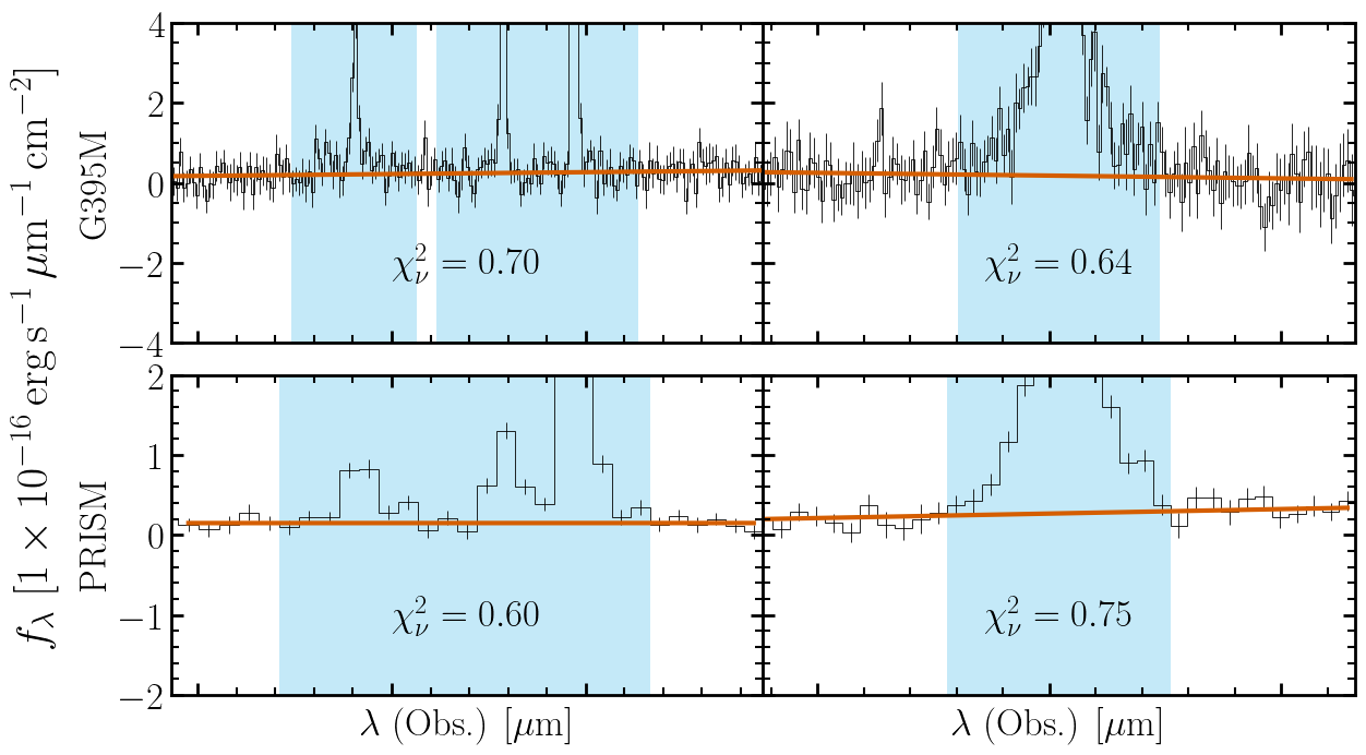
In this case, the errors are overestimated (\(\chi^2_\nu < 1\)) so the error bars are scaled down in each region for each spectrum by the appropriate factor.

Step 6 — Fit with SVI

For this example we will run the model with SVI as it is fast with relatively good accuracy.

See Sampling & Optimization for NUTS, nested sampling, GPU acceleration, and using SVI to initialize NUTS. See Building the Model for the ModelBuilder API.

builder = model.ModelBuilder(filtered_lines, filtered_cont, spectra)
model_fn, model_args = builder.build()

guide = infer.autoguide.AutoMultivariateNormal(model_fn)
optimizer = optim.Adam(0.01)
svi = infer.SVI(model_fn, guide, optimizer, loss=infer.Trace_ELBO())
svi_result = svi.run(jax.random.PRNGKey(0), 10000, model_args, progress_bar=False)

samples = guide.sample_posterior(
    jax.random.PRNGKey(1), svi_result.params, sample_shape=(500,)
)

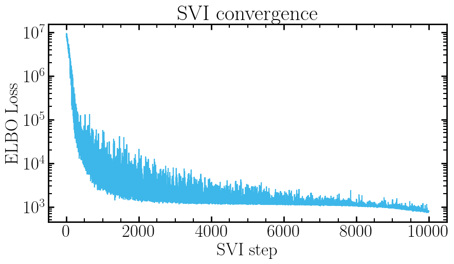
# Plot ELBO convergence
fig, ax = pyplot.subplots(figsize=(10, 5))
ax.plot(svi_result.losses)
ax.set(xlabel='SVI step', ylabel='ELBO Loss', title='SVI convergence', yscale='log')
pyplot.show()

Step 7 — Extract Results and Plot

make_parameter_table() returns a flat Table with one row per posterior sample. make_spectra_tables() returns a dict keyed by spectrum name, with wavelength, continuum, and per-line model predictions per spectrum. Passing percentiles only returns the percentiles, not the samples. Returned tables are also in physical units based on the input. Pass return_hdul=True to get an HDUList directly for saving to disk.

See Results and Output for FITS output, rest equivalent widths, and evaluating the model at arbitrary samples.

percentiles = [0.16, 0.5, 0.84]
param_table = results.make_parameter_table(samples, model_args, percentiles=percentiles)
spectra_tables = results.make_spectra_tables(
    samples,
    model_args,
    insert_nan=True,  # Insert NaN between regions for neater plotting
    percentiles=percentiles,
)

print(param_table)

percentile        z_shared        ...   pix_offset_PRISM      r_scale_a
                                  ...
---------- ---------------------- ... ------------------- ------------------
      0.16 0.00020234843685002247 ... 0.22201127501013662 0.7879232491190432
       0.5 0.00030945451782435297 ... 0.24001769269134832 0.8063055455835592
      0.84 0.00043086761669425494 ... 0.25786077708555744 0.8286449274539228

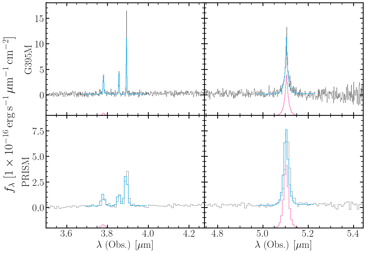
Multi-panel figure showing data and median model for both gratings.

fig, axes = pyplot.subplots(2, 2, figsize=(14, 10), sharex='col')
fig.subplots_adjust(hspace=0, wspace=0)

xlims = [
    (4500 * (1 + zspec) / 1e4, 5500 * (1 + zspec) / 1e4),
    (6100 * (1 + zspec) / 1e4, 7000 * (1 + zspec) / 1e4),
]

for row, s in enumerate(spectra):
    tab = spectra_tables[s.name]
    median_model = tab['model_total'][:, 1]
    for col, ax in enumerate(axes[row]):
        ax.step(s.wavelength, s.flux, where='mid', color='k', lw=0.6, alpha=0.7)
        ax.step(tab['wavelength'], median_model, where='mid', color='C0', lw=1.5)

        if row == 0:
            ax.set(xlim=xlims[col], ylim=[-4, 18])
        else:
            ax.set(
                ylim=[-2, 9], xlabel=rf'$\lambda$ (Obs.) [{prism_spectrum.unit:latex}]'
            )
        if col == 0:
            ax.set(ylabel=s.name)
        else:
            ax.set(yticklabels=[])

        for line_name in 'ab':
            sub = 2 if row else 4
            ax.step(
                tab['wavelength'],
                tab[f'H{line_name}_broad'][:, 1].value - sub,
                where='mid',
                color='C1',
                lw=1,
            )

fig.supylabel(rf'$f_\lambda$ [{prism_spectrum.flux_unit:latex_inline}]')
pyplot.show()

Step 8 — Model Diagnostics

NumPyro’s log_likelihood() and log_density() make it straightforward to compute log-likelihoods, log-posteriors, and information criteria directly from the posterior samples we already have.

See Results and Output (Model Diagnostics section) for the full reference, including ArviZ integration for PSIS-LOO and multi-model comparison.

import jax.numpy as jnp
from numpyro.infer.util import log_density, log_likelihood

Degrees of freedom — count the free scalar parameters in the compiled model. This traces the model once (no sampling) and is useful as a quick sanity check before comparing models.

from unite.results import count_parameters

n_params = count_parameters(model_fn, model_args)
print(f'Free parameters: {n_params}')

Free parameters: 16

Reduced chi-square — uses the median model from spectra_tables (Step 7) against the scaled errors. NaN rows inserted by insert_nan=True are automatically excluded by the finite mask.

chi2_total = 0.0
n_pixels_total = 0
for t in spectra_tables.values():
    obs = t['observed_flux']
    err = t['scaled_error']
    med = t['model_total'][:, 1]  # median (50th percentile, could do it from max logL
    valid = jnp.isfinite(med)
    resid = (obs[valid] - med[valid]) / err[valid]
    chi2_total += (resid**2).sum()
    n_pixels_total += valid.sum()

dof = n_pixels_total - n_params
chi2_red = chi2_total / dof
print(
    f'χ²_nu = {chi2_red:.3f}  ({n_pixels_total} pixels - {n_params} params = {dof} DoF)'
)

χ²_nu = 5.329  (390 pixels - 16 params = 374 DoF)

Log-likelihood — log_likelihood() returns a dict mapping each observed site (one per spectrum) to an array of shape (n_samples, n_pixels). Summing over pixels gives the total per-sample log-likelihood.

log_liks = log_likelihood(model_fn, samples, model_args)

ll_obs = jnp.hstack(list(log_liks.values()))
total_ll = ll_obs.sum(-1)
print(f'Mean log-likelihood: {total_ll.mean():.2f}')

Mean log-likelihood: -787.17

Log-posterior (unnormalized log-joint density: log p(θ, data)). log_density() traces the full model including priors, so this includes both the likelihood and the prior log-probabilities. jax.jit(jax.vmap(...)) compiles once and evaluates all samples in parallel.

def _log_joint(sample):
    ld, _ = log_density(model_fn, (model_args,), {}, sample)
    return ld


# log_density only accepts one sample, so we vectorize with JAX
log_joint = jax.jit(jax.vmap(_log_joint))(samples)
print(f'Mean log-posterior: {log_joint.mean():.2f}')

Mean log-posterior: -807.87

WAIC (Widely Applicable Information Criterion). Computed per-pixel from the log-likelihood array — lower is better. lppd is the log pointwise predictive density. Lower WAIC is better.

lppd = jnp.sum(jax.nn.logsumexp(ll_obs, axis=0) - jnp.log(ll_obs.shape[0]))
p_waic = jnp.sum(jnp.var(ll_obs, axis=0))
waic = -2.0 * (lppd - p_waic)
print(f'WAIC: {waic:.2f}')

WAIC: 4575.22