Note

Go to the end to download the full example code.

Full Generic Workflow¶

A complete unite fit on simulated data using a fully custom spectrograph. No real data files required — we generate a synthetic spectrum in the first step.

We fit H$\alpha$ + [NII]$\lambda\lambda$6549,6585 with a narrow + broad decomposition on a linear continuum. The focus here is on customisation: building a disperser from scratch, loading a spectrum from raw arrays, and exercising the full inference and diagnostics pipeline. The emission-line and continuum configuration, inference, and result-extraction steps are identical to the NIRSpec tutorial — refer back to those sections for deeper discussion.

Step 0 — Imports and Setup¶

import astropy.units as u
import jax
import jax.numpy as jnp
import numpy as np
from matplotlib import pyplot
from numpyro import infer

from unite import continuum, line, model, prior, results, spectrum

pyplot.style.use('unite.mplstyle')

Step 1 — Configure the Disperser¶

GenericDisperser accepts arbitrary JAX-jittable callables for R(λ) and dλ/dpix(λ), making it suitable for any instrument whose response cannot be expressed as a constant or simple grid. Here we model a low-resolution spectrograph whose resolving power rises linearly from R = 800 at 6200 Å to R = 1200 at 6900 Å — realistic for, e.g., a longslit spectrograph with a grism tilted off blaze.

The pixel scale is uniform (constant dλ/dpix), so we hard-code it from the grid spacing.

If your instrument has a constant R or a simple pixel-sampled grid, use SimpleDisperser instead — it only needs a wavelength array and one of R, dlam, or dvel. Built-in dispersers (e.g. G395M, SDSSDisperser) are drop-in replacements — the rest of the workflow is identical.

An optional RScale calibration token is attached to leave the effective resolution as a free parameter in the model. This is useful when the true LSF width is uncertain (slit filling, seeing, etc.).

See Instruments & Spectrum Loading for the full disperser and calibration token reference.

from unite.instrument import RScale
from unite.instrument.generic import GenericDisperser
from unite.spectrum import Spectrum

WL_MIN, WL_MAX, N_PIX = 6200.0, 6900.0, 500
dlam_pix = (WL_MAX - WL_MIN) / (N_PIX - 1)  # Å/pixel (uniform grid)

disperser = GenericDisperser(
    R_func=lambda w: 800.0 + (w - WL_MIN) / (WL_MAX - WL_MIN) * 400.0,
    dlam_dpix_func=lambda w: jnp.full_like(w, dlam_pix),
    unit=u.AA,
    name='custom_grism',
    r_scale=RScale(prior=prior.TruncatedNormal(low=0.7, high=1.3, loc=1.0, scale=0.1)),
)

# For a constant-R instrument the simpler alternative is:
# disperser = SimpleDisperser(wavelength=wavelength_q, R=1000.0, name='custom_grism')

print(disperser)

<unite.instrument.generic.GenericDisperser object at 0x77bd3fe53b60>

Step 2 — Simulate and Load the Spectrum¶

We generate a 500-pixel synthetic spectrum with:

A narrow H$\alpha$ + [NII] triplet (FWHM ≈ 300 km/s intrinsic, convolved with the LSF)
A broad H$\alpha$ component (FWHM ≈ 2000 km/s, mimicking a broad-line region)
A gently sloping linear continuum
Gaussian noise at S/N ≈ 5 per pixel on the continuum

Spectrum takes pixel edges (low, high) rather than centers, which unite uses for exact pixel integration. Flux and error must be Quantity with f-lambda units.

See Instruments & Spectrum Loading (Generic Dispersers section) for the full Spectrum API.

rng = np.random.default_rng(0)

wavelength_q = np.linspace(WL_MIN, WL_MAX, N_PIX) * u.AA
wl = wavelength_q.value

# LSF FWHM at Ha for the disperser (R ~ 1030 at 6563 Å)
R_ha = 800.0 + (6563.0 - WL_MIN) / (WL_MAX - WL_MIN) * 400.0
lsf_fwhm_ha = 6563.0 / R_ha  # Å

# Narrow component: 300 km/s intrinsic, convolved with LSF
c_kms = 299792.458
fwhm_narrow_aa = 6563.0 * 200.0 / c_kms
sigma_narrow = np.sqrt(fwhm_narrow_aa**2 + lsf_fwhm_ha**2) / (
    2 * np.sqrt(2 * np.log(2))
)

# Broad component: 2000 km/s (much wider than LSF, so LSF convolution is negligible)
sigma_broad = 6563.0 * 2000.0 / c_kms / (2 * np.sqrt(2 * np.log(2)))

true_flux = (
    # Narrow Ha + [NII] doublet (1:3 ratio for NII 6549:6585 is approximate)
    60.0 * np.exp(-0.5 * ((wl - 6563.0) / sigma_narrow) ** 2)
    + 15.0 * np.exp(-0.5 * ((wl - 6549.0) / sigma_narrow) ** 2)
    + 45.0 * np.exp(-0.5 * ((wl - 6585.0) / sigma_narrow) ** 2)
    # Broad Ha
    + 20.0 * np.exp(-0.5 * ((wl - 6563.0) / sigma_broad) ** 2)
)
true_continuum = 20.0 + 0.008 * (wl - 6550.0)
noise_sigma = 3.0

flux_arr = (true_flux + true_continuum + rng.normal(0, noise_sigma, N_PIX)) * 1e-17
error_arr = np.full(N_PIX, noise_sigma * 1e-17)

flux_q = flux_arr * u.erg / u.s / u.cm**2 / u.AA
error_q = error_arr * u.erg / u.s / u.cm**2 / u.AA

# Pixel edges from the uniform grid
half = 0.5 * dlam_pix
low_q = (wl - half) * u.AA
high_q = (wl + half) * u.AA

spec = Spectrum(
    low=low_q,
    high=high_q,
    flux=flux_q,
    error=error_q,
    disperser=disperser,
    name='custom',
)
print(spec)

Spectrum 'custom': 500 px, λ ∈ [6199, 6901] Angstrom [calibrated]

Plot the raw spectrum to guide model design.

fig, ax = pyplot.subplots(figsize=(10, 8))
ax.step(wl, flux_q.value * 1e17, where='mid', color='k', lw=0.8, label='Simulated data')
ax.fill_between(
    wl,
    (flux_q - error_q).value * 1e17,
    (flux_q + error_q).value * 1e17,
    alpha=0.3,
    color='k',
)
ax.set(
    xlabel=r'$\lambda$ [\AA]',
    ylabel=r'$f_\lambda$ [$10^{-17}$ erg s$^{-1}$ cm$^{-2}$ \AA$^{-1}$]',
    title=r'Synthetic H$\alpha$ + [NII] — narrow + broad',
)
pyplot.tight_layout()
# pyplot.show()

$Synthetic H$\alpha$ + [NII] — narrow + broad$

Step 3 — Configure the Emission Lines¶

We build the same narrow + broad decomposition as the NIRSpec tutorial:

Narrow: shared redshift and FWHM across H$\alpha$ and the [NII] doublet
[NII] doublet: approximate 1:3 strength ratio via strength
Broad: FWHM prior that must exceed narrow + 300 km/s, keeping the two components identifiable

See Line Configuration for the full line and profile reference and Priors for dependent priors and all supported prior types.

line_configuration = line.LineConfiguration()

z_common = line.Redshift('common', prior=prior.Uniform(-0.001, 0.001))
fwhm_narrow = line.FWHM('narrow', prior=prior.Uniform(50, 300))
fwhm_broad = line.FWHM('broad', prior=prior.Uniform(fwhm_narrow + 150, 3000))

# Narrow Ha
line_configuration.add_line(
    'Ha',
    6563.0 * u.AA,
    profile='Gaussian',
    redshift=z_common,
    fwhm_gauss=fwhm_narrow,
    flux=line.Flux(prior=prior.Uniform(0, 3)),
)

# [NII] doublet — fixed 1:3 flux ratio
line_configuration.add_lines(
    'NII',
    np.array([6549.0, 6585.0]) * u.AA,
    profile='Gaussian',
    redshift=z_common,
    fwhm_gauss=fwhm_narrow,
    strength=[1.0, 3.0],
    flux=line.Flux(prior=prior.Uniform(0, 3)),
)

# Broad Ha — independent flux, Gaussian profile
line_configuration.add_line(
    'Ha_broad',
    6563.0 * u.AA,
    profile='Gaussian',
    redshift=z_common,
    fwhm_gauss=fwhm_broad,
    flux=line.Flux(prior=prior.Uniform(0, 3)),
)

print(line_configuration)

LineConfiguration: 4 lines, 3 flux / 1 z / 2 profile params

  Name      Wavelength        Profile   Redshift  Params             Flux/Tau       zorder  Strength
  --------  ----------------  --------  --------  -----------------  -------------  ------  --------
  Ha        6563.00 Angstrom  Gaussian  z_common  fwhm_gauss_narrow  flux_Ha        0       1.00
  NII_6549  6549.00 Angstrom  Gaussian  z_common  fwhm_gauss_narrow  flux_NII_6549  0       1.00
  NII_6585  6585.00 Angstrom  Gaussian  z_common  fwhm_gauss_narrow  flux_NII_6549  0       3.00
  Ha_broad  6563.00 Angstrom  Gaussian  z_common  fwhm_gauss_broad   flux_Ha_broad  0       1.00

  Redshift:
    z_common  Uniform(low=-0.001, high=0.001)

  Params (fwhm_gauss):
    fwhm_gauss_narrow  Uniform(low=50.0, high=300.0)
    fwhm_gauss_broad   Uniform(low=(narrow + 150.0), high=3000.0)

  Flux:
    flux_Ha        Uniform(low=0.0, high=3.0)
    flux_NII_6549  Uniform(low=0.0, high=3.0)
    flux_Ha_broad  Uniform(low=0.0, high=3.0)

Step 4 — Configure the Continuum¶

Auto-generate a single linear continuum window around all line centers.

See Continuum Configuration for manual regions, other continuum forms (power law, Chebyshev, blackbody, …), and parameter sharing across regions.

cc = continuum.ContinuumConfiguration.from_lines(
    line_configuration.centers, width=15_000 * u.km / u.s, form=continuum.Linear()
)
print(cc)

ContinuumConfiguration: 1 region(s), 3 parameter(s), zorder=0

  Range                                    Unit      Form      Parameters
  ---------------------------------------  --------  --------  ----------------------------
  [6385.161655541047, 6749.7389675159875]  Angstrom  Linear()  scale_a, angle_a, norm_wav_a

  Parameters:
    scale_a     Uniform(low=0.0, high=2.0)
    angle_a     Uniform(low=-1.5707963267948966, high=1.5707963267948966)
    norm_wav_a  Fixed(6567.450311528517)

Step 5 — Prepare the Spectra¶

prepare() filters lines and continuum regions to those observable in the spectrum. compute_scales() estimates the flux normalization and, with error_scale=True, per-region error rescaling.

See Building the Model for details on coverage filtering, flux scales, and the continuum diagnostic plots.

spectra = spectrum.Spectra([spec], redshift=0.0)

filtered_lines, filtered_cont = spectra.prepare(line_configuration, cc)

spectra.compute_scales(
    filtered_lines,
    filtered_cont,
    line_mask_width=3_000 * u.km / u.s,
    box_width=2_000 * u.km / u.s,
    error_scale=True,
)

print(f'Line scale:      {spectra.line_scale:.4g}')
print(f'Continuum scale: {spectra.continuum_scale:.4g}')

Line scale:      3.816e-14 erg / (s cm2)
Continuum scale: 1.995e-16 erg / (Angstrom s cm2)

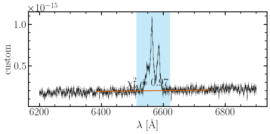
Inspect the continuum fit before committing to inference. The broad component is not masked here — only the narrow-line region is excluded. A good fit (χ²ν ≈ 1) confirms the scale estimation is reliable.

fig, axes = pyplot.subplots(
    len(list(spectra)),
    len(filtered_cont),
    figsize=(10, 4 * len(list(spectra))),
    sharey='row',
    sharex='col',
)
axes = np.atleast_2d(axes)
fig.subplots_adjust(hspace=0.1, wspace=0)

for row, s in enumerate(spectra):
    diag = s.scale_diagnostic
    wl_s = s.wavelength
    mask = diag.line_mask

    for col, reg in enumerate(diag.regions):
        ax = axes[row, col]
        ax.step(wl_s, s.flux, where='mid', color='k', lw=0.6)
        ax.errorbar(
            wl_s,
            s.flux,
            yerr=s.error,
            fmt='none',
            ecolor='k',
            elinewidth=0.6,
            capsize=0,
        )
        masked = np.where(mask)[0]
        for group in np.split(masked, np.where(np.diff(masked) != 1)[0] + 1):
            if len(group):
                ax.axvspan(
                    s.low[group[0]], s.high[group[-1]], color='C0', alpha=0.3, lw=0
                )
        ax.plot(wl_s[reg.in_region], reg.model_on_region, lw=2, color='C3')
        ax.text(
            0.5,
            0.25,
            rf'$\chi^2_\nu = {reg.chi2_red:.2f}$',
            ha='center',
            va='center',
            transform=ax.transAxes,
        )
        if col == 0:
            ax.set(ylabel=s.name)
        if row == len(list(spectra)) - 1:
            ax.set(xlabel=r'$\lambda$ [\AA]')

# pyplot.show()

Step 6 — Sample with MCMC¶

ModelBuilder assembles the NumPyro model. We now will sample the posterior with MCMC.

See Sampling & Optimization for more information on NUTS, SVI, nested sampling, GPU acceleration, and using SVI to warm-start NUTS. See Building the Model for the full ModelBuilder API. Notice the warning about not enough devices.

builder = model.ModelBuilder(filtered_lines, filtered_cont, spectra)
model_fn, model_args = builder.build()

kernel = infer.NUTS(
    model_fn, dense_mass=True
)  # dense_mass=True helps with correlated parameters
mcmc = infer.MCMC(
    kernel, num_warmup=500, num_samples=1000, num_chains=2, progress_bar=False
)
mcmc.run(jax.random.PRNGKey(0), model_args)
samples = mcmc.get_samples()

/home/docs/checkouts/readthedocs.org/user_builds/unite/checkouts/v2.7.1/docs/tutorials/tutorial_generic.py:339: UserWarning: There are not enough devices to run parallel chains: expected 2 but got 1. Chains will be drawn sequentially. If you are running MCMC in CPU, consider using `numpyro.set_host_device_count(2)` at the beginning of your program. You can double-check how many devices are available in your system using `jax.local_device_count()`.
  mcmc = infer.MCMC(

Step 7 — Extract Results and Plot¶

make_parameter_table() returns physical-unit posteriors. make_spectra_tables() returns a dict keyed by spectrum name, decomposing the model into per-line and continuum contributions. Pass return_hdul=True to get an HDUList directly for saving to disk.

See Results and Output for FITS output, rest equivalent widths, and evaluating the model at arbitrary samples.

percentiles = np.array([0.16, 0.5, 0.84])
param_table = results.make_parameter_table(samples, model_args, percentiles=percentiles)
spectra_tables = results.make_spectra_tables(
    samples, model_args, insert_nan=True, percentiles=percentiles
)

print(param_table)

percentile         z_common        ... r_scale_custom_grism
                                   ...
---------- ----------------------- ... --------------------
      0.16 -2.7081152801171937e-05 ...   0.8946479695285291
       0.5 -1.3445290653616437e-05 ...   0.9935550191744951
      0.84   4.754369744506412e-07 ...   1.0977461952596232

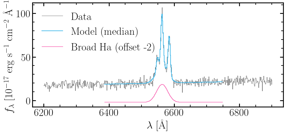
Plot data, total model, and the broad component individually.

fig, ax = pyplot.subplots(figsize=(10, 5))

tab = spectra_tables['custom']
median_model = tab['model_total'][:, 1]
broad = tab['Ha_broad'][:, 1]

ax.step(
    spec.wavelength,
    spec.flux * 1e17,
    where='mid',
    color='k',
    lw=0.6,
    alpha=0.7,
    label='Data',
)
ax.step(
    tab['wavelength'],
    median_model.value * 1e17,
    where='mid',
    color='C0',
    lw=1.5,
    label='Model (median)',
)
ax.step(
    tab['wavelength'],
    broad.value * 1e17 - 2,
    where='mid',
    color='C1',
    lw=1,
    label='Broad Ha (offset -2)',
)

ax.set(
    xlabel=r'$\lambda$ [\AA]',
    ylabel=r'$f_\lambda$ [$10^{-17}$ erg s$^{-1}$ cm$^{-2}$ \AA$^{-1}$]',
)
ax.legend()
pyplot.tight_layout()
# pyplot.show()


from numpyro.infer.util import log_density, log_likelihood

Degrees of freedom — count the free scalar parameters in the compiled model. This traces the model once (no sampling) and is useful as a quick sanity check before comparing models.

from unite.results import count_parameters

n_params = count_parameters(model_fn, model_args)
print(f'Free parameters: {n_params}')

Free parameters: 9

Reduced chi-square — uses the median model from spectra_tables (Step 7) against the scaled errors. NaN rows inserted by insert_nan=True are automatically excluded by the finite mask.

chi2_total = 0.0
n_pixels_total = 0
for t in spectra_tables.values():
    obs = t['observed_flux']
    err = t['scaled_error']
    med = t['model_total'][:, 1]  # median (50th percentile, could do it from max logL
    valid = jnp.isfinite(med)
    resid = (obs[valid] - med[valid]) / err[valid]
    chi2_total += (resid**2).sum()
    n_pixels_total += valid.sum()

dof = n_pixels_total - n_params
chi2_red = chi2_total / dof
print(
    f'χ²_nu = {chi2_red:.3f}  ({n_pixels_total} pixels - {n_params} params = {dof} DoF)'
)

χ²_nu = 1.102  (259 pixels - 9 params = 250 DoF)

Log-likelihood — log_likelihood() returns a dict mapping each observed site (one per spectrum) to an array of shape (n_samples, n_pixels). Summing over pixels gives the total per-sample log-likelihood.

log_liks = log_likelihood(model_fn, samples, model_args)

ll_obs = jnp.hstack(list(log_liks.values()))
total_ll = ll_obs.sum(-1)
print(f'Mean log-likelihood: {total_ll.mean():.2f}')

Mean log-likelihood: 126.35

Log-posterior (unnormalized log-joint density: log p(θ, data)). log_density() traces the full model including priors, so this includes both the likelihood and the prior log-probabilities. jax.jit(jax.vmap(...)) compiles once and evaluates all samples in parallel.

def _log_joint(sample):
    ld, _ = log_density(model_fn, (model_args,), {}, sample)
    return ld


# log_density only accepts one sample, so we vectorize with JAX
log_joint = jax.jit(jax.vmap(_log_joint))(samples)
print(f'Mean log-posterior: {log_joint.mean():.2f}')

Mean log-posterior: 114.94

WAIC (Widely Applicable Information Criterion). Computed per-pixel from the log-likelihood array — lower is better. lppd is the log pointwise predictive density. Lower WAIC is better.

lppd = jnp.sum(jax.nn.logsumexp(ll_obs, axis=0) - jnp.log(ll_obs.shape[0]))
p_waic = jnp.sum(jnp.var(ll_obs, axis=0))
waic = -2.0 * (lppd - p_waic)
print(f'WAIC: {waic:.2f}')

WAIC: -242.24

Total running time of the script: (0 minutes 59.635 seconds)

Gallery generated by Sphinx-Gallery